In article Statistics with R (Part I), we walked-through the basic statistics calculation using R and also regression models incl. linear regression, multiple regression, logistic regression and Poisson regression. In this part, we will continue to explore more complicated analysis including Analysis of Covariance, Time Series Analysis, Decision Tree and Random Forest, etc.
Analysis of Covariance
Analysis of covariance (ANCOVA) is a general linear model which blends ANOVA and regression. ANCOVA evaluates whether the means of a dependent variable (DV) are equal across levels of a categorical independent variable (IV) often called a treatment, while statistically controlling for the effects of other continuous variables that are not of primary interest, known as covariates (CV) or nuisance variables. Mathematically, ANCOVA decomposes the variance in the DV into variance explained by the CV(s), variance explained by the categorical IV, and residual variance. Intuitively, ANCOVA can be thought of as 'adjusting' the DV by the group means of the CV(s).
*Definition from Wikipedia.
There are two main functions in R related to such kind of analysis:
- aov(): Fit an analysis of variance model by a call to lm for each level.
- anova(): Compute analysis of variance (or deviance) tables for one or more fitted model objects.
Let's have a look at the following example (script R41.ANCOVA.R):
result1 <- aov(mpg~hp*am,data = mtcars)
print(summary(result1))

result2 <- aov(mpg~hp+am,data = mtcars)
print(summary(result2))

print(anova(result1,result2))
The analysis result is like the following:
> print(anova(result1,result2))
Analysis of Variance Table

Model 1: mpg ~ hp * am
Model 2: mpg ~ hp + am
  Res.Df RSS Df Sum of Sq  F Pr(>F)
1     28 245
2     29 245 -1  -0.00525  0   0.98
As the p-value is greater than 0.05, the interaction between horse power and transmission type is not significant. So the mileage per gallon will depend in a similar manner on the horse power of the car in both auto and manual transmission mode.
Time series analysis
Time series is a series of data elements in which each element is associated with a timestamp. One example is the amount of transactions for each bank account on different days of each month.
In R, time series object can be created using the following function:
ts(data, start, end, frequency)
The details for the parameters:
- data: a vector or matrix containing the values.
- start: the start time for the first observation.
- end: the end time for the last observation.
- frequency: the number of observations per unit time.
For parameter 'frequency', the values can be:
- 12: data sampled for every month of a year.
- 4: data sampled for every quarter of a year.
- 6: data sampled for every 10 minutes of an hour.
- 24*6: data sampled for every 10 minutes of a day.
The following code snippet (script R42.TimeSeries.R) creates a time series object using generated data:
(sales1 <- abs(rnorm(20, mean=30, sd=5)))
(sales2 <- abs(rnorm(20, mean=20, sd=3)))
(sales3 <- abs(rnorm(20, mean=10, sd=6)))

# Time series
(sales.timeseries <- ts(matrix(c(sales1,sales2,sales3), nrow=20),start = c(2017,1),frequency = 12))

# Plot
# colors
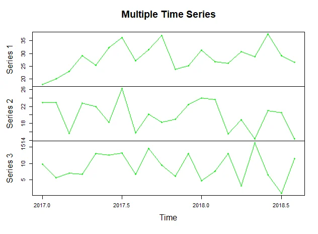
plot(sales.timeseries, main="Multiple Time Series", type="o", col="green")
The plot looks like the following:
Decision tree
A decision tree is a graphical depiction of a decision and every potential outcome or result of making that decision. The nodes represent an state or choice and the edges of the graph represent the decision rules or conditions.
Here are some of the example usages of decision tree:
- predicting an email as spam or not spam
- predicting a banking account transaction is fraud or not.
One of the R packages for creating decision tree is 'party'. The function for creating a decision tree object is like this:
ctree(formula, data)
- formula: a formula describing the independent variables and dependent variable.
- data: the name of the data set
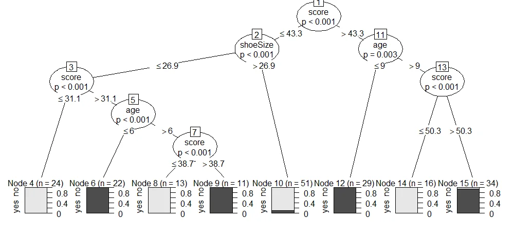
The following script (script R43.DecisionTree.R) uses ctreefunction to create two decision trees and then plot the results:
library(party)

# Native speaker example
(output.tree <- ctree(
  nativeSpeaker ~ age + shoeSize + score,
  data = readingSkills))

plot(output.tree)

# Iris example
cdt <- ctree(Species ~ . , iris)
plot(cdt)
The output trees look like the following screenshots:
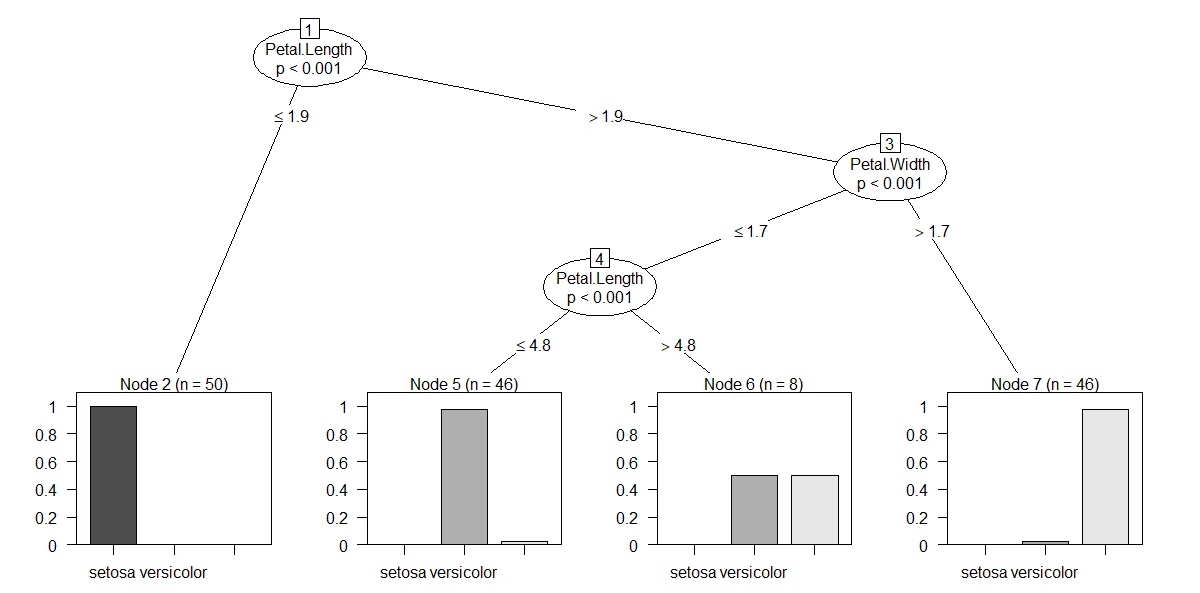
The above chart basically tells us that if the iris petal length <=1.9, it will be 100% categorized as setosa.
Random forest
In R, randomForest implements Breiman's random forest algorithm (based on Breiman and Cutler's original Fortran code) for classification and regression.
The function is defined as the following:
randomForest(formula, data)
- formula: a formula describing the independent variables and dependent variable.
- data: the name of the data set.
To visualize random forest, forestFloorpackage can be used.
The following code snippet provides an example of random forest:
require(randomForest)

(
  output.forest <- randomForest(Species ~ .,
                              data = iris,  keep.inbag=T)
)

# This is the extractor function for variable importance measures as produced by randomForest.
print(importance(output.forest,type = 2))

# visualize it:
require(forestFloor)

(X = iris[,!names(iris)=="Species"])
floor <- forestFloor(output.forest, X,  keep.inbag=T)

# plot
# colors
colors <- terrain.colors(5)

# 2D
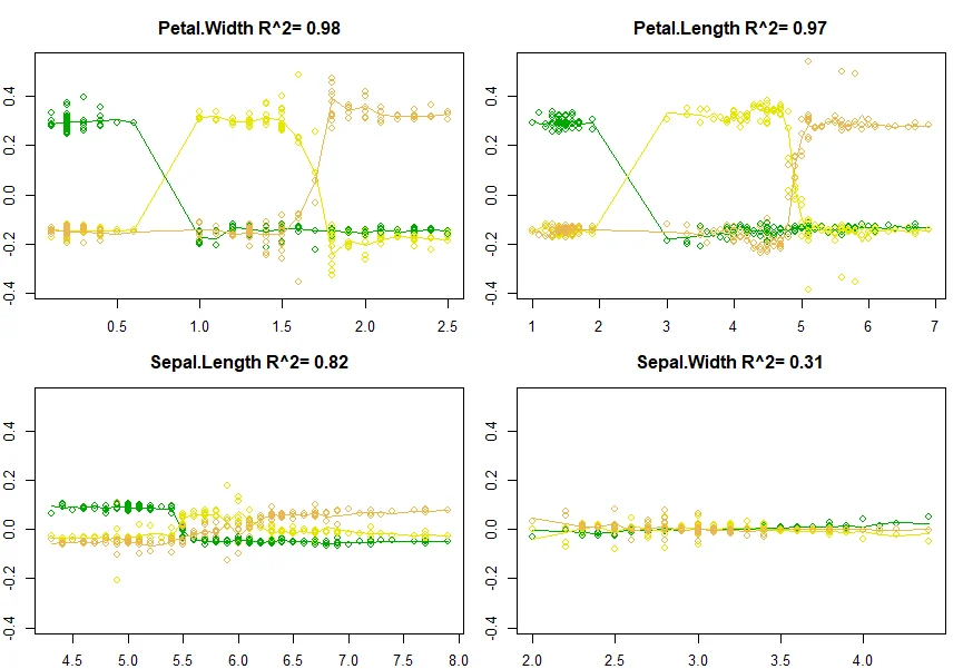
plot(floor, col=colors)
# 3D
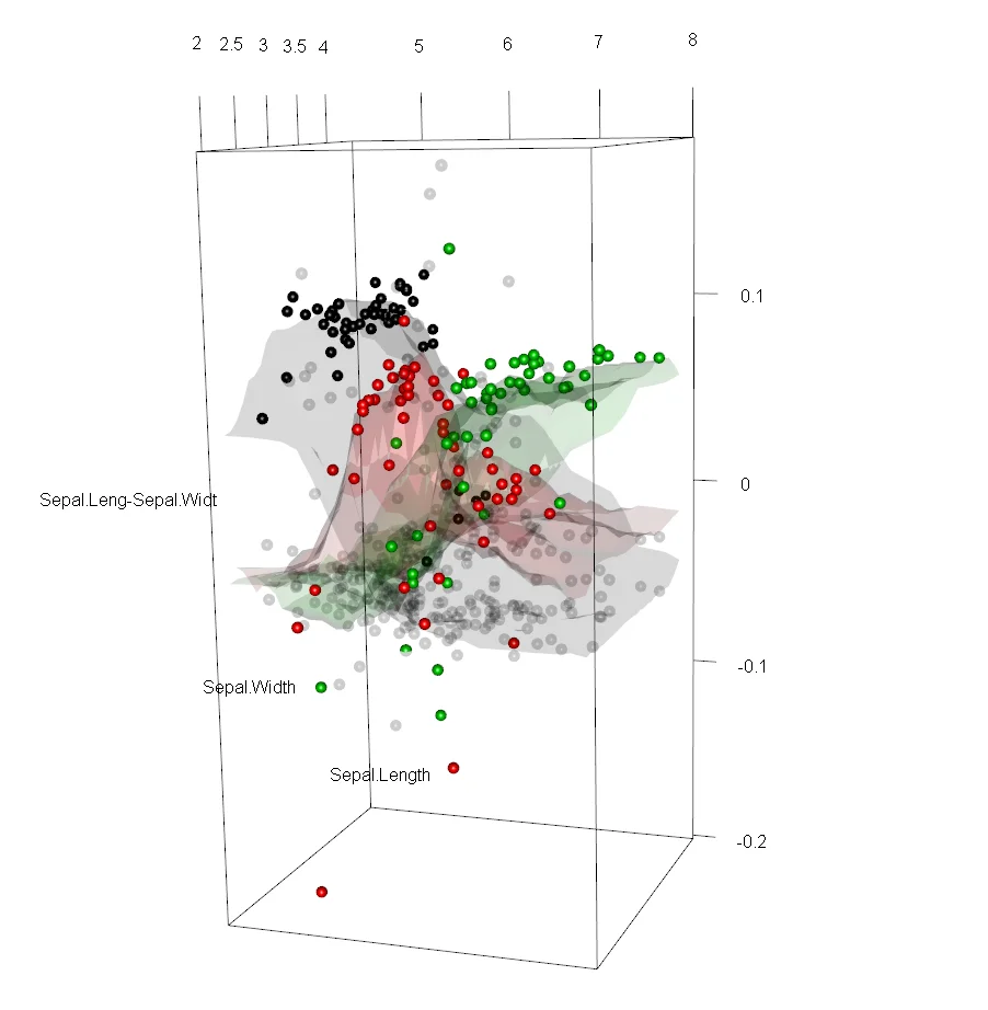
show3d(floor, col=colors)
The 2D plot looks like the following screenshot:
Other analysis
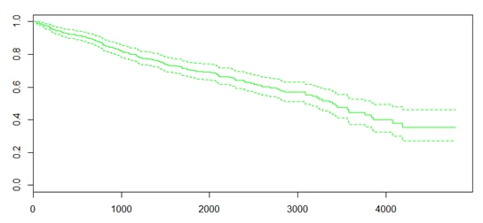
R also supports many other types of analysis. For example, Survival Analysis is a type of analysis to predict the time when a specific event is going to occur. In R, package 'survival' can be used for this type of analysis.
The following is an example of survival analysis:
require('survival')

# Create the survival object.
# y~1 fits a model with no effects (only the intercept)
(sf <- survfit(Surv(pbc$time,pbc$status == 2)~1))
plot(sf, col="green")
Another type of analysis is Chi-Square test, which is a statistical method to test if two categorical variables have a significant correlation between them. In R, the function to perform Chi-Square test is chisq.test(data).
Summary
With R's broad libraries, we can perform various analysis against our data. Understanding each analysis' usages and objectives are critical to choose the right model and formula to resolve our business problems.