Geoanalytics is a powerful field that combines geographic location with data analysis. It provides a visual perspective, uncovers hidden insights, and enhances decision-making by integrating geography with data analysis. This article shows you how to use Python package geopandas to analyze and visualize ABS (Australian Bureau of Statistics) published public data.
About geopandas
Python package geopandas is an open-source Python library that extends the capabilities of pandas (a popular data science library) to handle geospatial data. It builds on top of pandas and shapely. It allows you to work with both tabular data (like pandas DataFrames) and geometries (such as points, lines, and polygons). There are several key components in this library:
- GeoDataFrame: A GeoPandas GeoDataFrame is a subclass of pandas DataFrame that can store geometry columns and perform spatial operations.
- GeoSeries: A GeoSeries is a subclass of pandas Series that handles geometries.
- You can have multiple columns with geometries in a GeoDataFrame, each potentially in a different coordinate reference system (CRS).
For easily data analytics, I recommend you to use a notebook environment to run the Python code, for example, Jupyter Notebook.
Install the package
Run the following command to install required Python packages into your environment:
pip install geopandas
pip install matplotlib
Note - matplotlib will be required to plotting in this tutorial.
Download ABS SA4 digital boundary data
ABS publishes different levels of digital boundary data as part of Australian Statistical Geography Standard (ASGS) Edition 3. You can download them from this official page. ABS provides different levels of digital boundary data as the following image shows:
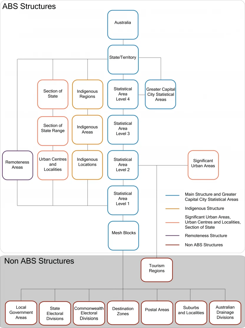 *Image from Australian Statistical Geography Standard (ASGS) Edition 3, July 2021 - June 2026 | Australian Bureau of Statistics (abs.gov.au).
We will use data set Statistical Areas Level 1 - 2021 - Shapefile.
Extract the data
After downloading the zip file, extract it into a folder. I am extracting it to a subfolder named data:
Mode LastWriteTime Length Name ---- ------------- ------ ---- -ar--- 20/04/2021 8:31 AM 39272153 SA1_2021_AUST_GDA2020.dbf -ar--- 20/04/2021 8:31 AM 160 SA1_2021_AUST_GDA2020.prj -ar--- 20/04/2021 8:31 AM 153904384 SA1_2021_AUST_GDA2020.shp -ar--- 20/04/2021 8:31 AM 494860 SA1_2021_AUST_GDA2020.shx -a---- 21/06/2021 8:01 AM 25585 SA1_2021_AUST_GDA2020.xml
It contains several files that will be used later.
Read shapefile to GeoDateFrame
The above published dataset is in format of shapefile. We can use geopandas to read it directly.
import geopandas as gpd
shp_file_path = 'data/SA1_2021_AUST_GDA2020.shp'
data = gpd.read_file(shp_file_path)
The related attributes information in file *.dbf will also be read.
Explore the data
We can use the common pandas DataFrame methods to explore the data.
data.columns
The above code prints out the following column list information of the DataFrame:
Index(['SA1_CODE21', 'CHG_FLAG21', 'CHG_LBL21', 'SA2_CODE21', 'SA2_NAME21', 'SA3_CODE21', 'SA3_NAME21', 'SA4_CODE21', 'SA4_NAME21', 'GCC_CODE21', 'GCC_NAME21', 'STE_CODE21', 'STE_NAME21', 'AUS_CODE21', 'AUS_NAME21', 'AREASQKM21', 'LOCI_URI21', 'geometry'], dtype='object')
The last column geometry is in format of WKT.
print(data.loc[0, 'geometry'])
The following is the WKT extract from the first geometry.
POLYGON ((149.8911094722651 -35.0898882056091, 149.89181447220685 -35.08951620566876, 149.8924794621867 -35.0888981957232,...-35.09042220555832, 149.89074246229112 -35.090115205578286, 149.8911094722651 -35.0898882056091))
The numbers are coordinates of SA1 10102100702.
data.shape
The above line will print out the following information:
(61845, 18)
It means there are 61845 geometries in this data set at SA1 level across Australia.
data.iloc[1]
The above code prints out the attributes (columns) of the first row in the DataFrame:
SA1_CODE21 10102100702 CHG_FLAG21 0 CHG_LBL21 No change SA2_CODE21 101021007 SA2_NAME21 Braidwood SA3_CODE21 10102 SA3_NAME21 Queanbeyan SA4_CODE21 101 SA4_NAME21 Capital Region GCC_CODE21 1RNSW GCC_NAME21 Rest of NSW STE_CODE21 1 STE_NAME21 New South Wales AUS_CODE21 AUS AUS_NAME21 Australia AREASQKM21 229.7459 LOCI_URI21 http://linked.data.gov.au/dataset/asgsed3/SA1/... geometry POLYGON ((149.73421044994282 -35.3675691937016... Name: 1, dtype: object
This give you a hint about what the data looks like.
data[data['STE_NAME21'] == "Victoria"]['SA4_NAME21'].unique()
The above code prints out the SA4 list in state Victoria:
array(['Ballarat', 'Bendigo', 'Geelong', 'Hume', 'Latrobe - Gippsland', 'Melbourne - Inner', 'Melbourne - Inner East', 'Melbourne - Inner South', 'Melbourne - North East', 'Melbourne - North West', 'Melbourne - Outer East', 'Melbourne - South East', 'Melbourne - West', 'Mornington Peninsula', 'North West', 'Shepparton', 'Warrnambool and South West', 'Migratory - Offshore - Shipping (Vic.)', 'No usual address (Vic.)'], dtype=object)
Convert WKT to geojson
geopandas provides built-in function that can be used to save the DataFrame to geojson file. The following is an example:
shp_file_path = 'data/SA1_2021_AUST_GDA2020.shp'
geojson_file_path = 'data/SA1_2021_AUST_GDA2020.geojson'
data = gpd.read_file(shp_file_path)
data.to_file(geojson_file_path, driver='GeoJSON')
The driver='GeoJSON' argument ensures that the output file format is GeoJSON.
If you just want to convert a single WKT string to GeoJSON format, you can shapely directly:
from shapely.geometry import mapping
# Convert the geometry to GeoJSON
geojson = mapping(data.loc[0, 'geometry'])
print(geojson)
The output looks like the following:
{'type': 'Polygon', 'coordinates': (((149.8911094722651, -35.0898882056091), .... }
Plot examples
Now let's start to plot the GeoDataFrame. Similarly as pandas DataFrame, we can directly plot with built in methods.
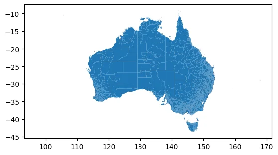
Plot the whole DataFrame
data.plot()
The output looks like the following screenshot:
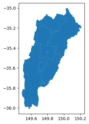
Plot the first 10 geometries
data.head(10).plot()
The output:
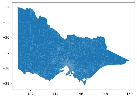
Plot Victoria state
data[data['STE_NAME21'] == "Victoria"].plot()
The above code filters on state name and then plot all the geometries in Victoria state. The output looks like the following screenshot:
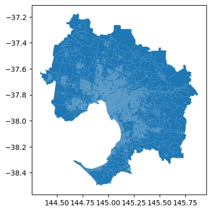
Plot Greater Melbourne area
print(data[data['GCC_NAME21'] == "Greater Melbourne"]['SA4_NAME21'].unique())
greater_melbourne = data[data['GCC_NAME21'] == "Greater Melbourne"]
greater_melbourne.plot()
The output looks like the following:
['Melbourne - Inner' 'Melbourne - Inner East' 'Melbourne - Inner South' 'Melbourne - North East' 'Melbourne - North West' 'Melbourne - Outer East' 'Melbourne - South East' 'Melbourne - West' 'Mornington Peninsula']
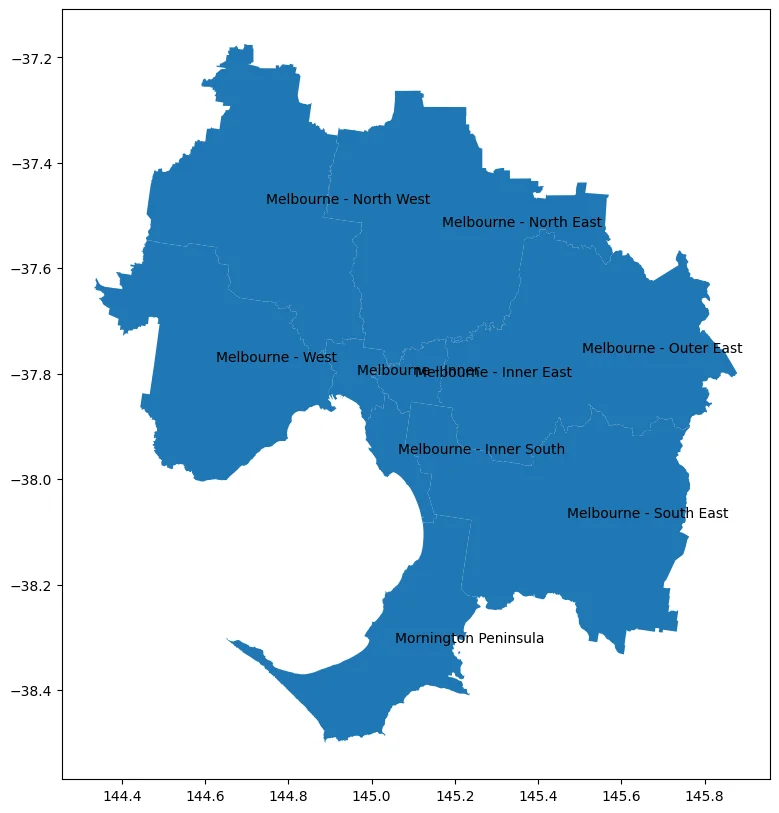
Dissolve from SA1 to SA4 level
For SA4 level data, there are in total 61845 geometries and the map looks very busy. We can use dissolve method to create higher level maps directly.
Note - You can also read from SA4 digital boundary file directly to plot.
The following code snippet dissolve by column SA4_NAME21. It also adds labels to the center of the geometry.
import matplotlib.pyplot as plt

# Create a new figure with a specific size (width, height)
fig, ax = plt.subplots(figsize=(15, 10))

# Dissolve the data by 'SA4_NAME21' and plot it
dissolved = greater_melbourne.dissolve(by='SA4_NAME21')
dissolved.plot(ax=ax)

# Add labels
for x, y, label in zip(dissolved.geometry.centroid.x, dissolved.geometry.centroid.y, dissolved.index):
    plt.text(x, y, label)

plt.show()
The output looks like the following screenshot:
Plot with data metrics
It doesn't provide any insights directly if we just plot with geometries. Now let's add some data metrics to visualize on the map. We will use another ABS dataset of population from Census 2021.
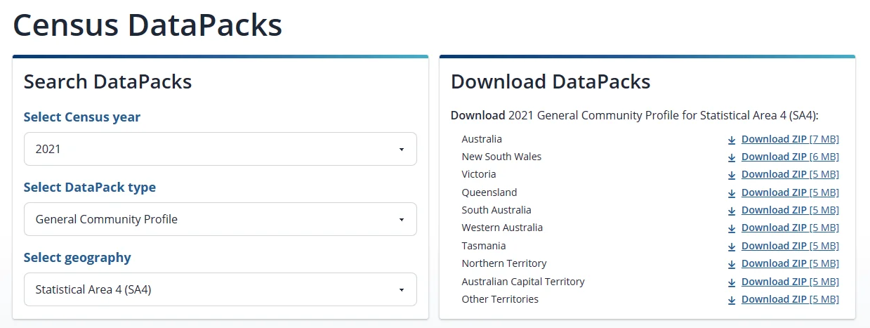
Download the census data
Go to page Census DataPacks | Australian Bureau of Statistics (abs.gov.au). Select SA4 as the following screenshot shows:
 Download the Victoria data from this link: https://www.abs.gov.au/census/find-census-data/datapacks/download/2021\_GCP\_SA4\_for\_VIC\_short-header.zip.
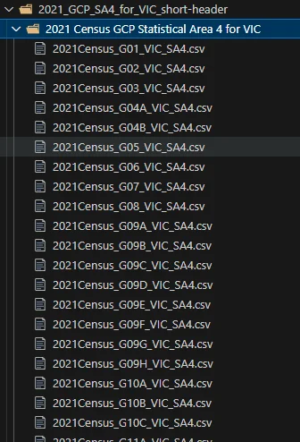
Extract the data to a directory. I'm saving the data to a directory named '2021_GCP_SA4_for_VIC_short-header' in my project folder.
The folder contains a number of CSV files:
Download the Victoria data from this link: https://www.abs.gov.au/census/find-census-data/datapacks/download/2021\_GCP\_SA4\_for\_VIC\_short-header.zip.
Extract the data to a directory. I'm saving the data to a directory named '2021_GCP_SA4_for_VIC_short-header' in my project folder.
The folder contains a number of CSV files:
Read the census data as DataFrame
Now we can easily read the data as DataFrame using pandas:
# Read population data from ABS SA4 level
import pandas as pd
import glob

# Get a list of all CSV files in the directory
csv_files = glob.glob('2021_GCP_SA4_for_VIC_short-header/2021 Census GCP Statistical Area 4 for VIC/*.csv')

# Read each CSV file into a DataFrame and store them in a list
dfs = [pd.read_csv(f) for f in csv_files]

# Concatenate all dataframes in the list into a single DataFrame
df_census = pd.concat(dfs, ignore_index=True)
df_census.shape
The output:
(2261, 16294)
There are 2261 records in the DataFrame object. Let's further explore the dataset using the following code:
df_census.columns
It prints out the following:
Index(['SA4_CODE_2021', 'Tot_P_M', 'Tot_P_F', 'Tot_P_P', 'Age_0_4_yr_M', 'Age_0_4_yr_F', 'Age_0_4_yr_P', 'Age_5_14_yr_M', 'Age_5_14_yr_F', 'Age_5_14_yr_P', ... 'Three_meth_Tot_three_meth_P', 'Worked_home_M', 'Worked_home_F', 'Worked_home_P', 'Did_not_go_to_work_M', 'Did_not_go_to_work_F', 'Did_not_go_to_work_P', 'Method_travel_to_work_ns_M', 'Method_travel_to_work_ns_F', 'Method_travel_to_work_ns_P'], dtype='object', length=16294)
We will primarily use column SA4_CODE_2021 and Tot_P_P which represents SA4 code and total population accordingly.
df_census['SA4_CODE_2021']=df_census['SA4_CODE_2021'].astype(str)
df_census_subset = df_census[['SA4_CODE_2021', 'Tot_P_P']]
The above code snippet creates a subset and also convert column to SA4_CODE_2021 to object type so that we can join with our GeoDataFrame later.
Join the two DataFrames
greater_melbourne2 = greater_melbourne.merge(df_census_subset, left_on='SA4_CODE21', right_on='SA4_CODE_2021', how='left')
greater_melbourne2 = greater_melbourne2.dropna()
The above code snippets joins the two dataset by column SA4_CODE21 and SA4_CODE_2021.
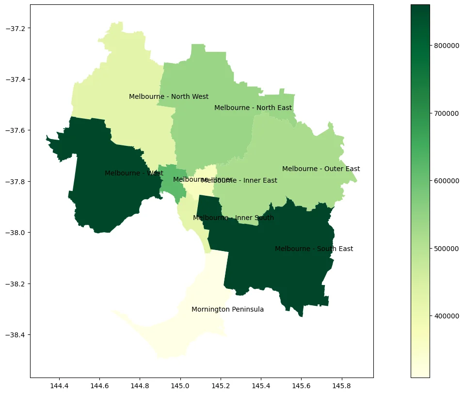
Plot the population metric
Now let's plot the populations of each SA4 area of Greater Melbourne region on a map:
import matplotlib.pyplot as plt

# Create a new figure with a specific size (width, height)
fig, ax = plt.subplots(figsize=(20, 10))

dissolved2 = greater_melbourne2.dissolve(by='SA4_NAME21')
dissolved2.plot(column='Tot_P_P', legend=True, ax=ax, cmap='YlGn')

# Add labels
for x, y, label in zip(dissolved2.geometry.centroid.x, dissolved2.geometry.centroid.y, dissolved2.index):
    plt.text(x, y, label)

plt.show()
It outputs the following chart:
Summary
As you can see, it is very easy and flexible to plot this the public Geo data. Have fun with GeoAnalytics!