Till now, we've gone through R programming basics, data types, packages and IDEs, data APIs to work with data sources and various plotting functions. Let's now dive into the most important part about statistics and modelling with R. After all, R was created for statistics.
warning Due to my limited knowledge in statistics, I cannot explain this part very well. If you find anything is not accurate or not clear, kindly point out and correct me.
Model formulae
A formula is typically of the form y ~ model:
- y: the analyzed response
- model: a set of terms separated with arithmetic symbols, for which some parameters are to be estimated.
The operators in a formula has different meaning compared those in expressions.
Function I can be used to include arithmetic operations. For example, y ~I(x1+x2) defines the model y = β(x1+x2)+α.
Formulae examples
The following table summarizes some of the model examples with their meaning.
| Model Example | Meaning |
|---|---|
| a+b | additive effects of a and of b |
| X | if X is a matrix, this specifies an additive effect of each of its columns, i.e. X[,1]+X[,2]+...+X[,ncol(X)]; some of the columns may be selected with numeric indices (e.g., X[,2:4]) |
| a:b | interactive effect between a and b |
| a*b | additive and interactive effects (identical to a+b+a:b) |
| poly(a, n) | polynomials of a up to degree n |
| ^n | includes all interactions up to level n, i.e. (a+b+c)^2 is identical to a+b+c+a:b+a:c+b:c |
| b %in% a | the effects of b are nested in a (identical to a+a:b, or a/b) |
| -b | removes the effect of b, for example: (a+b+c)^2-a:b is identical to a+b+c+a:c+b:c |
| -1 | y origin (Similar as above for y |
| 1 | y~1 fits a model with no effects (only the intercept) |
| offset(...) | adds an effect to the model without estimating any parameter (e.g., offset(3*x)) |
Basic statistics
The basic and frequently used statistics are mean, median, mode, max, min. R has functions available to calculate these stats:
| Stats | R function |
|---|---|
| Mean | <br>mean(x, trim = 0, na.rm = FALSE, ...)<br> |
| Median | <br>median(x, na.rm = FALSE) <br> |
| Mode | <br>unique<br>tabulate<br>which.max<br> |
| Max | <br>max()<br> |
| Min | <br>min()<br> |
The following code snippet (script R34.MeanMedianMode.R) shows examples of these functions:
> (x <- sample.int(100,size=70))
 [1] 40 85 91  8 68 23 62 47 81 28 92 39 98  5 66 70 96 44 74 16 88 51 65 63 46 32 95 36
[29] 34 21 49 99 43 48 90 20 53 86 55  6 26 31 73  2 97 18 22 41 35 72  7 67 57 93 37 71
[57] 24 94  4  9 83 54 14 75 69 29 19 13 79 80
>
> # mean
> mean(x)
[1] 51.5
>
> # median
> median(x)
[1] 50
>
> # mode
>
> x <- c(1,2,34,56,11,2,3,44,2,2,1,3,4,5)
>
> (uniqueX <- unique(x))
[1]  1  2 34 56 11  3 44  4  5
>
> (counts <- tabulate(match(x, uniqueX)))
[1] 2 4 1 1 1 2 1 1 1
>
> uniqueX[which.max(counts)]
[1] 2
>
>
> # max
> max(x)
[1] 56
>
> min(x)
[1] 1
>
Linear regression model
In Linear Regression these two variables are related through an equation, where exponent (power) of both these variables is 1.
In math, the model can be interpreted as: y = ax + b
- y: dependent variable (response variable).
- x: independent variable (more accurate: predictor variable).
- a and b: constants (coefficients)
In R, function lm() can be used to fit liner regression models. Function predict() can be used for prediction.
Example
The following code snippet (script R35.LinearModel.R) demonstrates how to fit a linear model and then use it for prediction:
# Linear model
x <- c(1:36)
y <- c(5357.04
       ,7027.80
       ,8705.19
       ,16066.75
       ,12172.68
       ,9136.14
       ,8512.92
       ,15706.47
       ,16755.14
       ,22666.99
       ,17025.84
       ,12769.38
       ,12880.56
       ,16468.92
       ,22402.77
       ,24597.30
       ,28641.60
       ,18066.75
       ,13525.20
       ,16468.92
       ,29357.64
       ,33030.66
       ,33733.44
       ,17238.00
       ,18099.90
       ,21852.48
       ,29463.72
       ,36193.17
       ,30789.72
       ,22754.16
       ,22402.77
       ,21640.32
       ,29755.44
       ,32352.14
       ,43983.42
       ,33733.44)

# Apply the lm() function
relation <- lm(y~x)
class(relation)
print(relation)

# Get the summary of linear model
summary(relation)

# predict
a <- data.frame(x = 37:42)
(b <- predict(relation, a))
class(b)
# Draw the chart

plot(x,y,col="green", main = "Sales & Period Index Regression", type="o")

plot(x,y,col="green", main = "Sales & Period Index Regression", xlab="Period Index", ylab="Sales ($)"
)
# drawline
abline(lm(y~x), col="blue")

plot(x,y,col="green", main = "Sales & Period Index Regression", xlab="Period Index", ylab="Sales ($)",
     abline(lm(y~x), col="blue"),xlim=c(1,42)
)

points(a$x,b,col="red", type="p")
The summary will show the model details:
> summary(relation)Call:lm(formula = y ~ x)Residuals: Min 1Q Median 3Q Max -8997 -4439 -616 4064 11238 Coefficients: Estimate Std. Error t value Pr(>|t|) (Intercept) 8145.0 1976.9 4.12 0.00023 ***x 702.9 93.2 7.54 9.3e-09 ***---Signif. codes: 0 ‘***’ 0.001 ‘**’ 0.01 ‘*’ 0.05 ‘.’ 0.1 ‘ ’ 1Residual standard error: 5810 on 34 degrees of freedomMultiple R-squared: 0.626, Adjusted R-squared: 0.615 F-statistic: 56.9 on 1 and 34 DF, p-value: 9.26e-09
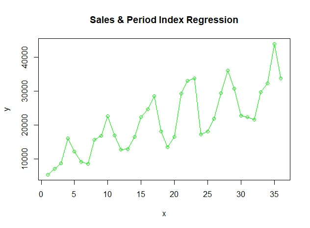
The input sales data looks like this:

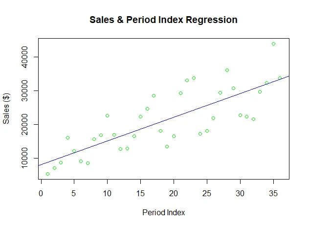
The fit model is plotted as a line chart (blue color):

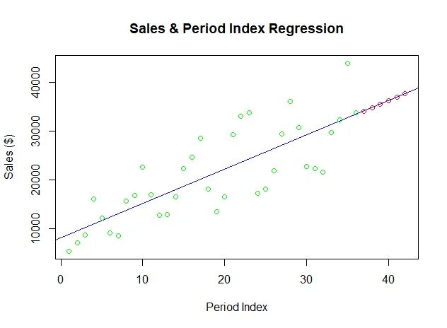
Finally the predicted values are also plotted on the graph (red color):

Multiple regression
Multiple regression is an extension of linear regression into relationship between more than two variables. In simple linear relation we have one predictor and one dependent variable, but in multiple regression we have more than one independent variable and one dependent variable.
In math, it can be interpreted as y = a + b1x1 + b2x2 +...bnxn:
- y: dependent variable.
- a, b1, b2...bn: the coefficients.
- x1, x2, ...xn: independent variables.
In R, multiple regression can be fit using functionlm(y ~ x1+x2+x3...,data).
The following code snippet (script R36.MultipleRegression.R) provides one example about multiple regression:
model <- lm(mpg~disp+hp+wt, data = mtcars[c("mpg","disp","hp","wt")]
)
print(model)
#
a <- coef(model)[1]
print(a)

(Xdisp <- coef(model)[2])
(Xhp <- coef(model)[3])
(Xwt <- coef(model)[4])
summary(model)
Function printoutputs the following detail:
Call:
lm(formula = mpg ~ disp + hp + wt, data = mtcars[c("mpg", "disp",
    "hp", "wt")])

Coefficients:
(Intercept)         disp           hp           wt
  37.105505    -0.000937    -0.031157    -3.800891
Logistic regression
The Logistic Regression is a regression model in which the dependent variable has categorical values such as True/False or 0/1. It actually measures the probability of a binary response as the value of dependent variable based on the mathematical equation relating it with the independent variables.
In math, it can be interpreted as y = 1/(1+e^-(a+b1x1+b2x2+b3x3+...)):
- y: dependent variable.
- x1,x2,…xn: independent variables.
- a and b: the coefficients (numeric constants).
In R, function glm(formula,data,family) can be used to fit the model. Parameter familyis a R object to specify the details of the model. Its value is binomial for logistic regression.
The following code snippet (script R37.LogisticRegression.R) shows an example of creating logistic regression model using glm function:
(
  model <- glm(am~cyl+hp+wt, data = mtcars[c("am","cyl","hp","wt")], family = binomial)
)

#
a <- coef(model)[1]
print(a)
(Xdisp <- coef(model)[2])
(Xhp <- coef(model)[3])
(Xwt <- coef(model)[4])

summary(model)
The fit model summary looks like the following:
> summary(model)

Call:
glm(formula = am ~ cyl + hp + wt, family = binomial, data = mtcars[c("am",
    "cyl", "hp", "wt")])

Deviance Residuals:
    Min       1Q   Median       3Q      Max
-2.1727  -0.1491  -0.0146   0.1412   1.2764

Coefficients:
            Estimate Std. Error z value Pr(>|z|)
(Intercept)  19.7029     8.1164    2.43    0.015 *
cyl           0.4876     1.0716    0.46    0.649
hp            0.0326     0.0189    1.73    0.084 .
wt           -9.1495     4.1533   -2.20    0.028 *
---
Signif. codes:  0 ‘***’ 0.001 ‘**’ 0.01 ‘*’ 0.05 ‘.’ 0.1 ‘ ’ 1

(Dispersion parameter for binomial family taken to be 1)

    Null deviance: 43.2297  on 31  degrees of freedom
Residual deviance:  9.8415  on 28  degrees of freedom
AIC: 17.84

Number of Fisher Scoring iterations: 8
Poisson regression
Poisson Regression involves regression models in which the response variable is in the form of counts and not fractional numbers. For example, the count of number of births or number of wins in a football match series. Also the values of the response variables follow a Poisson distribution.
In math, it can interpreted as log(y) = a + b1x1 + b2x2 + bnxn.....:
- y: dependent variable.
- a and b: the coefficients (numeric constants).
- x: independent variable.
In R, function **glm(formula,data,family)**can be used to fit a Poisson regression model. Parameter familyrepresents a R object to specify the details of the model. Its value is ‘Poisson’ for Poisson regression.
The following code snippet (script R40.PoissonRegression.R) provides one example about fitting Poisson regression model:
model <-glm(formula = breaks ~ wool+tension,
             data = warpbreaks,
             family = poisson)
(summary(model))