This article provides examples about plotting pie chart using pandas.DataFrame.plot function.
Prerequisites
The data I'm going to use is the same as the other article Pandas DataFrame Plot - Bar Chart. I'm also using Jupyter Notebook to plot them. The DataFrame has 9 records:
| DATE | TYPE | SALES |
|---|---|---|
| 0 | 2020-01-01 | TypeA |
| 1 | 2020-01-01 | TypeB |
| 2 | 2020-01-01 | TypeC |
| 3 | 2020-02-01 | TypeA |
| 4 | 2020-02-01 | TypeB |
| 5 | 2020-02-01 | TypeC |
| 6 | 2020-03-01 | TypeA |
| 7 | 2020-03-01 | TypeB |
| 8 | 2020-03-01 | TypeC |
Pie chart
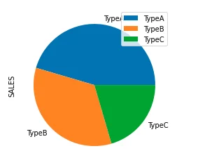
df.groupby(['TYPE']).sum().plot(kind='pie', y='SALES')
The above code outputs the following chart:
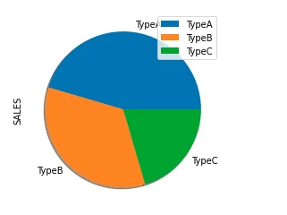
Shadow effect
df.groupby(['TYPE']).sum().plot(kind='pie', y='SALES', shadow = True)
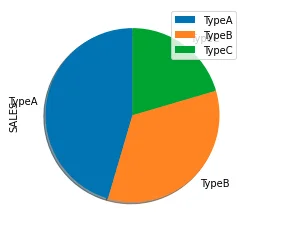
Start angle
df.groupby(['TYPE']).sum().plot(kind='pie', y='SALES', shadow = True, startangle=90)
Subplots (trellis)
We can also easily implement subplots/trellis charts. Let's add derive one more column on the existing DataFrame using the following code:
df['COUNT'] = df['SALES'] /100
df
The dataframe now looks like this:
| DATE | TYPE | SALES | COUNT | |
|---|---|---|---|---|
| 0 | 2020-01-01 | TypeA | 1000 | 10.0 |
| 1 | 2020-01-01 | TypeB | 200 | 2.0 |
| 2 | 2020-01-01 | TypeC | 300 | 3.0 |
| 3 | 2020-02-01 | TypeA | 700 | 7.0 |
| 4 | 2020-02-01 | TypeB | 400 | 4.0 |
| 5 | 2020-02-01 | TypeC | 500 | 5.0 |
| 6 | 2020-03-01 | TypeA | 300 | 3.0 |
| 7 | 2020-03-01 | TypeB | 900 | 9.0 |
| 8 | 2020-03-01 | TypeC | 100 | 1.0 |
Now we can plot the charts using the following code:
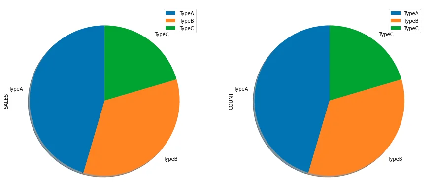
df.groupby(['TYPE']).sum().plot(kind='pie', subplots=True, shadow = True,startangle=90,figsize=(15,10))
In the above code, subplots=True parameter is used to plot charts on both SALES and COUNT metrics. The chart size is also increased using figsize parameter.
The chart now looks like the following screenshot:
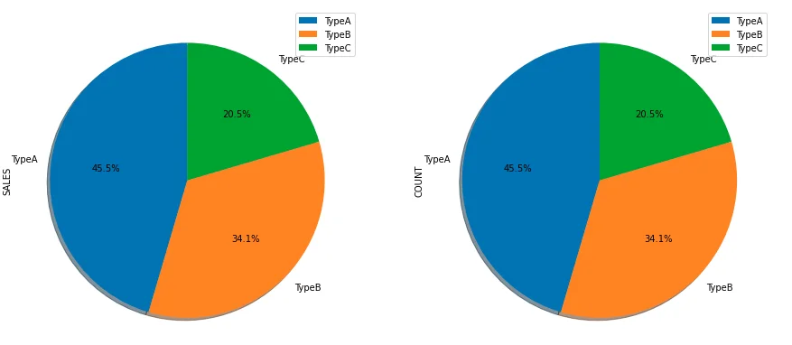
Add percentage
df.groupby(['TYPE']).sum().plot(kind='pie', subplots=True, shadow = True,startangle=90,
figsize=(15,10), autopct='%1.1f%%')